Visualizing annual sales change using a Waterfall Chart in Python with Plotly.

Because waterfalls are cleaner, clearer, calm and awesome!

A waterfall chart is a form of data visualization that helps in understanding the cumulative effect of sequentially introduced positive or negative values.

 These intermediate values can either be time-based or category based. The waterfall chart is also known as a flying bricks chart or Mario chart due to the apparent suspension of columns (bricks) in mid-air. Often in finance, it will be referred to as a bridge.

Photo by Robert Lukeman on Unsplash

Let’s take the following example:

I own a nationwide Salon company that offers salon services and also sells most of the cosmetic brands in Australia. I want to compare my sales between this year’s December Vs Last year’s December (Annual Sales Change). I’m more keen on knowing how my stores (branches) have performed for a particular cosmetic brand (Let’s say: LOreal). For you to get a clear understanding of this and the graph, Please take a look at the following image and this is what we are going to demonstrate at the end.

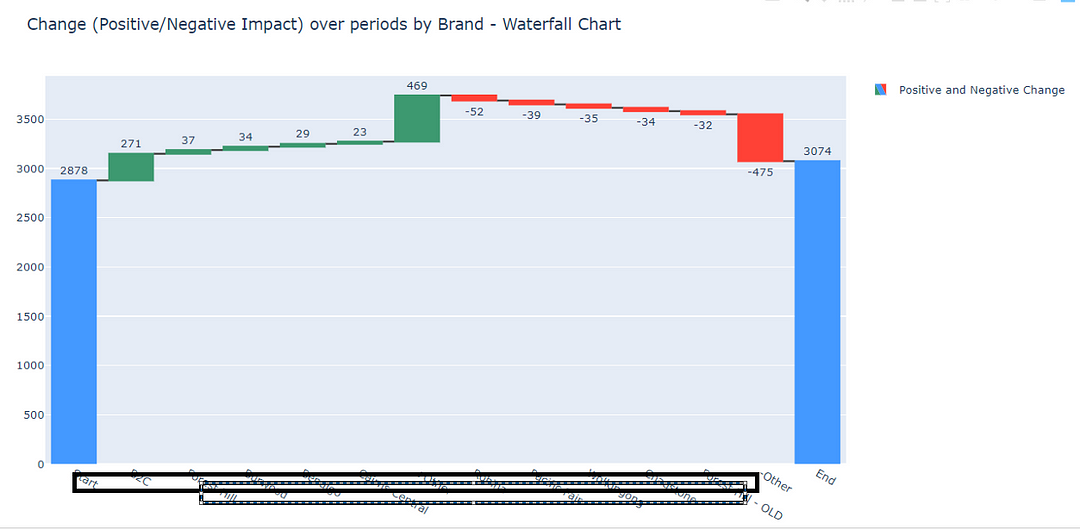
Brand: LOReal | Start — Last Year December | End — This Year December

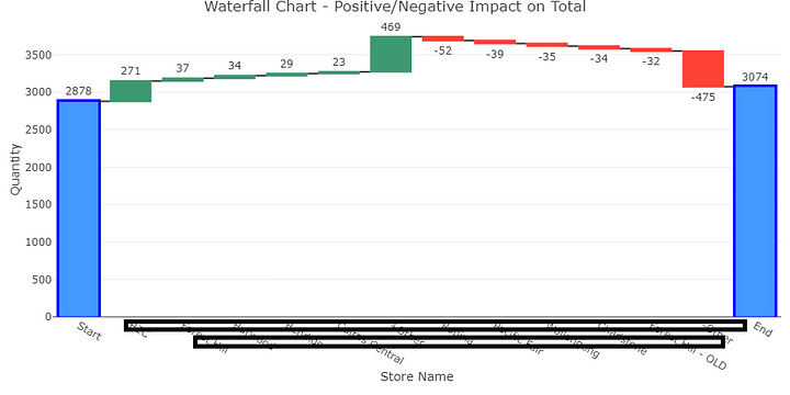
So what does this Waterfall chart tells you? By looking at this diagram you should get an idea like this:

My sales total quantity for last year’s December was 2878 LOreal products and the number went up to 3074 in this December. 198 more products to be more precise but how did this 198 calculated? Obvisouly there should be more sales in some particlar stores as well as less sales in some particular stores right? So in this graph, I can see which stores has a positive trend (Green Color) over the period and which has a negative trend (Red Color).

 

LET’S CODE!

This is the dataframe that has all the data for the brand LOreal.

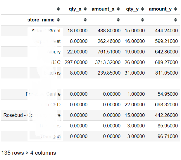
Note: x indicates the last season and y indicates this season.

First, We should get the Start and End value for the waterfall chart which means we need the sum of these numeric columns.

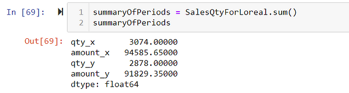
Which will give us the Quantity and Amount for the Dec 2019 and Dec 2018.

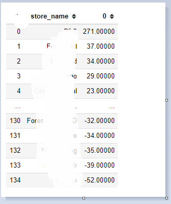
I want to focus on quantity so I need to create a new column with the change amount so run a python script to get (qty_x -qty_y) the difference and sort the column by high to low. I’ll name this DataFrame01

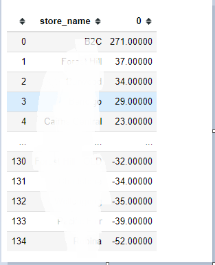
Column 0 indicates the change for each branch name.

Starting from now I’ll guide you step by step on how to create our waterfall chart.

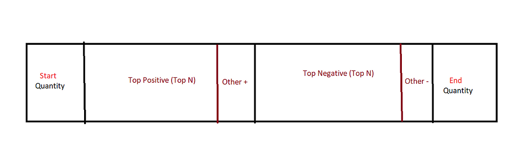
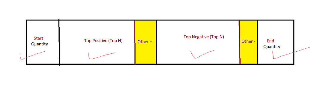
My target is to create a dataframe which has the first row as the starting total quantity which means last year’s Total Qty and then top positive changes will display in next 5 rows (Top 5) and the rest will sum up to a one row named +Others and then Top Negative 5 then the other negative numbers will sum up to a one row named -Others and the last row is the End total quantity which is this year’s Total Qty.

End look at my dataframe: Look at this illustration to get a clear idea

---

Step 01

In order to achieve the above dataframe, I’m going to create 4 different dataframes and in the end I’m going to concatenate them together.

I. dfQtyRowPeriod01

II. topPositive

III. topNegative.

IV. dfQtyRowPeriod02

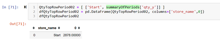
Get the start value from summaryOfPeriods (Earlier coding Step)

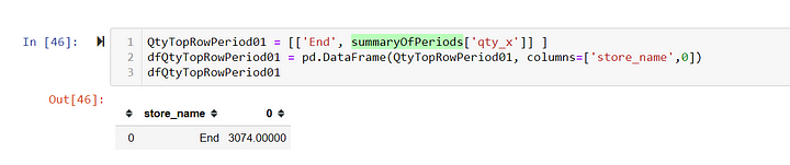
Get End value:

Ok, so we have created two separate dataframes that have the information we need regarding the start/end total quantity values.

Step 02

Ok, let’s take a look at our DataFrame01. (I’ll name this resultqty from now onwards)

Then the next step is to build the top positive and top negative dataframes separately.

#Positive Change and Negative Change in to seprate variables
PositiveChange = resultqty[resultqty[0] > 0] 
NegativeChange = resultqty[resultqty[0] < 0]

And get top N from each dataframe.

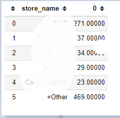
#positive top N
positive5 = PositiveChange.head(5)
positive5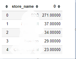

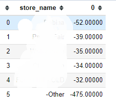
#Negative top N
negative5 = NegativeChange.sort_values(False).head(5)
negative5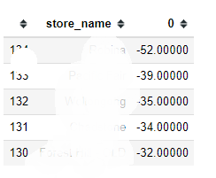

So far, we have covered the Start, Top Positive (5), Top negative (5) and End data frames for our final dataframe. What’s left is to aggregate the rest of the positives and negatives.

Progress Check

Step 03 — Aggregating the rest of Positive/Negatives

• Create two dataframes excluding the first 5 positive and negative values.

#rest of the negatives/positives
restNegatives = NegativeChange.sort_values(False)[5:]
restPositives = PositiveChange[5:]

• Then, Get the sum of each dataframe.

#sum of the rest
sumOfRestPositives = restPositives.sum()
sumOfRestNegatives = restNegatives.sum()

• Append the Sum value to topPositive and topNegative dataframes

topPositive = positive5.append(sumOfRestPositives, ignore_index= True)
topNegative = negative5.append(sumOfRestNegatives, ignore_index= True)

So now you have added a new row (Row 6) which has the total Positives and negatives but the Store Name column looks super freaky so we have to deal with this! (Look for yourself) :D

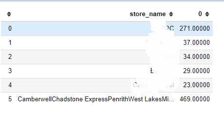
• Modify the Row 6th first column name.

topPositive['store_name'][5] = '+Other'
topNegative['store_name'][5] = '-Other'

• And print topPositive and topNegative to make sure we have done it properly.

Step 04 — Concat Them

• Now, Concat the above two dataframes together.

mergeofposandneg =pd.concat([topPositive,topNegative])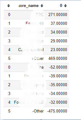

• NOW, Remember the first two dataframes we’ve created? Good. Let’s concat them all in this order:

FinalMergeTable =pd.concat([dfQtyTopRowPeriod02,mergeofposandneg,dfQtyTopRowPeriod01])
FinalMergeTable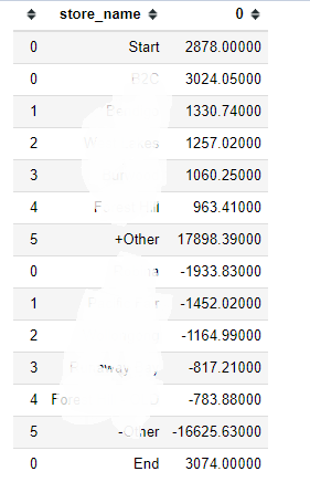

STEP 04 — Waterfall Chart using Plotly

I recommend you all to refer to this quick documentation and try a few graohs by yourself to get familiar with terms and attributes of Plotly.

IMPORTANT: You should obviously look into these ascribes

1. name
2. measure
3. x,y
4. textPosition
5. text
6. connector

import plotly.graph_objects as go

fig = go.Figure(go.Waterfall(
    name = "Positive and Negative Change",
    measure = ["absolute","relative","relative","relative","relative","relative","relative","relative","relative","relative","relative","relative","relative","total"], #6
    x = FinalMergeTable['store_name'], #6
    textposition = "outside",
    text = FinalMergeTable[0],
    y = FinalMergeTable[0],
    connector = {"line":{"color":"rgb(63, 63, 63, 0.5)"}},
) )

fig.update_layout(  
        title = "Change (Positive/Negative Impact) over periods by Brand - Waterfall Chart",
        showlegend = True, width=1200, height = 600
)

fig.show()

So just like that, You will finally get the waterfall chart like this:

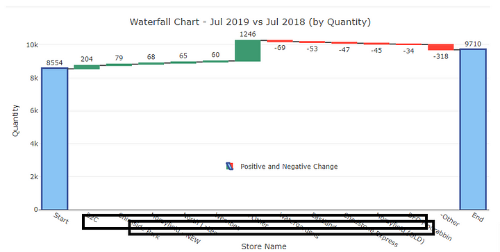
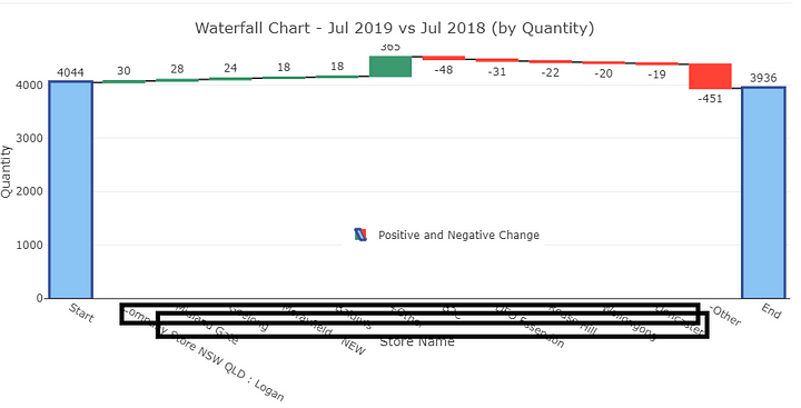
And there are some other examples I’ve tested trying different brands. (Dummy Locations)

Thank you and let me know if anything’s off or not clear, I’m happy to explain this again and again.

---

Keen on getting to know me and my work? Click here for more!

How to think like a Data Scientist (Secret to a data-driven mindset)
If you have read my previous article "Becoming a Data Scientist (Zero to Hero)", Consider this as the second part of…www.jayasekara.blog